
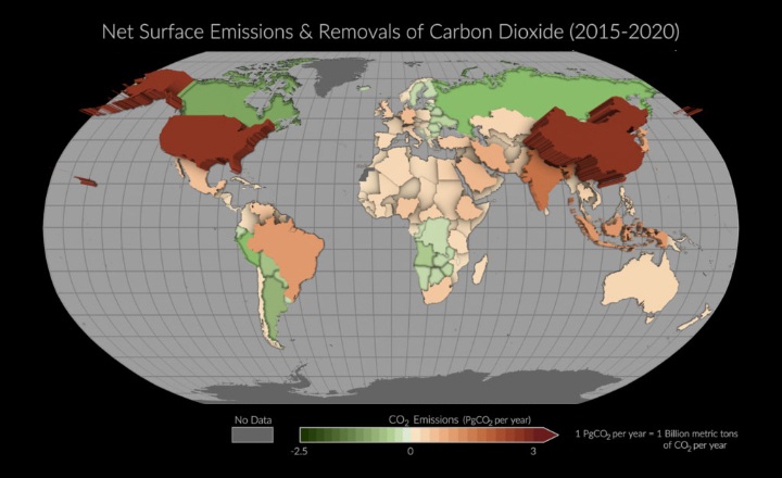
Un satélite de observación de la Tierra de la NASA ha ayudado a los investigadores a rastrear las emisiones de dióxido de carbono de más de 100 países de todo el mundo. El proyecto piloto ofrece una nueva y poderosa mirada al dióxido de carbono que se emite en estos países y cuánto de él es eliminado de la atmósfera por los bosques y otros “sumideros” que absorben carbono dentro de sus fronteras. Los hallazgos demuestran cómo las herramientas basadas en el espacio pueden respaldar los conocimientos sobre la Tierra a medida que las naciones trabajan para lograr los objetivos climáticos. Los cambios en las reservas de carbono de los ecosistemas terrestres dan como resultado emisiones y absorciones de CO2. Estos pueden ser impulsados por actividades antropogénicas (p. ej., deforestación), procesos naturales (p. ej., incendios) o en respuesta al aumento de CO2 (p. ej., fertilización con CO2). El documento de la referencia describe un conjunto de datos de emisiones y absorciones de CO2 derivadas de las observaciones atmosféricas de CO2. Este conjunto de datos piloto informa las capacidades actuales y los desarrollos futuros hacia los sistemas de verificación y monitoreo de arriba hacia abajo. Es interesante notar la escasa contribución de nuestro país al stock global de CO2.
We demonstrate how the dataset presented here can be compared with NGHGIs reported under the UNFCCC, which were downloaded from https://di.unfccc.int/flex_annex1 (last access: 6 February 2023). We also refer the reader to Chap. 6.10.2 in vol. 1 of IPCC (2019) for additional discussion of comparing top-down estimates with NGHGIs. The fossil fuel emissions in Byrne et al. (2022) can be compared with the combined emissions from the energy and IPPU (Energy+IPPU) categories. In both cases, these estimates account for anthropogenic CO2 emissions from the burning of fossil fuels and production of cement and other materials. We expect these estimates to generally be in good agreement, as they are similarly based on bottom-up accounting for national totals. However, the estimates may diverge when there are missing activity data, particularly in non-Annex 1 countries and more recent years (Andrew, 2020).
ΔCloss can be compared to the combined emissions and removals from the agriculture, LULUCF and waste (Agr+LULUCF+Waste) categories. These quantities are not identical, with the most important difference being that NGHGIs are only for managed land, while ΔCloss includes both managed and unmanaged lands. Therefore, caution is needed for parties with large unmanaged land areas (e.g., Canada or the Russian Federation). Another difference from NGHGIs is that ΔCloss implicitly includes deposition of carbon in water body sediments within a country (such as lakes). However, this is expected to be a small contribution. Similarly, volcanic CO2 emissions are implicitly included in ΔCloss but are also believed to be small contributions (global subaerial volcanic CO2 emissions are ∼0.05 Pg CO2 yr−1, Fischer et al., 2019). It is worth noting that NGHGIs require estimates of turnover times for wood products in producing countries, as these can have lifetimes of decades to centuries (see Appendix 3a.1 of Penman et al., 2003). No such estimate is needed for the top-down methods, as emissions from decaying wood products will be implicitly incorporated in NCE. Therefore, top-down methods only need to account for the lateral movement of wood products from the region where the carbon is sequestered to the region where the wood products are used and decompose.
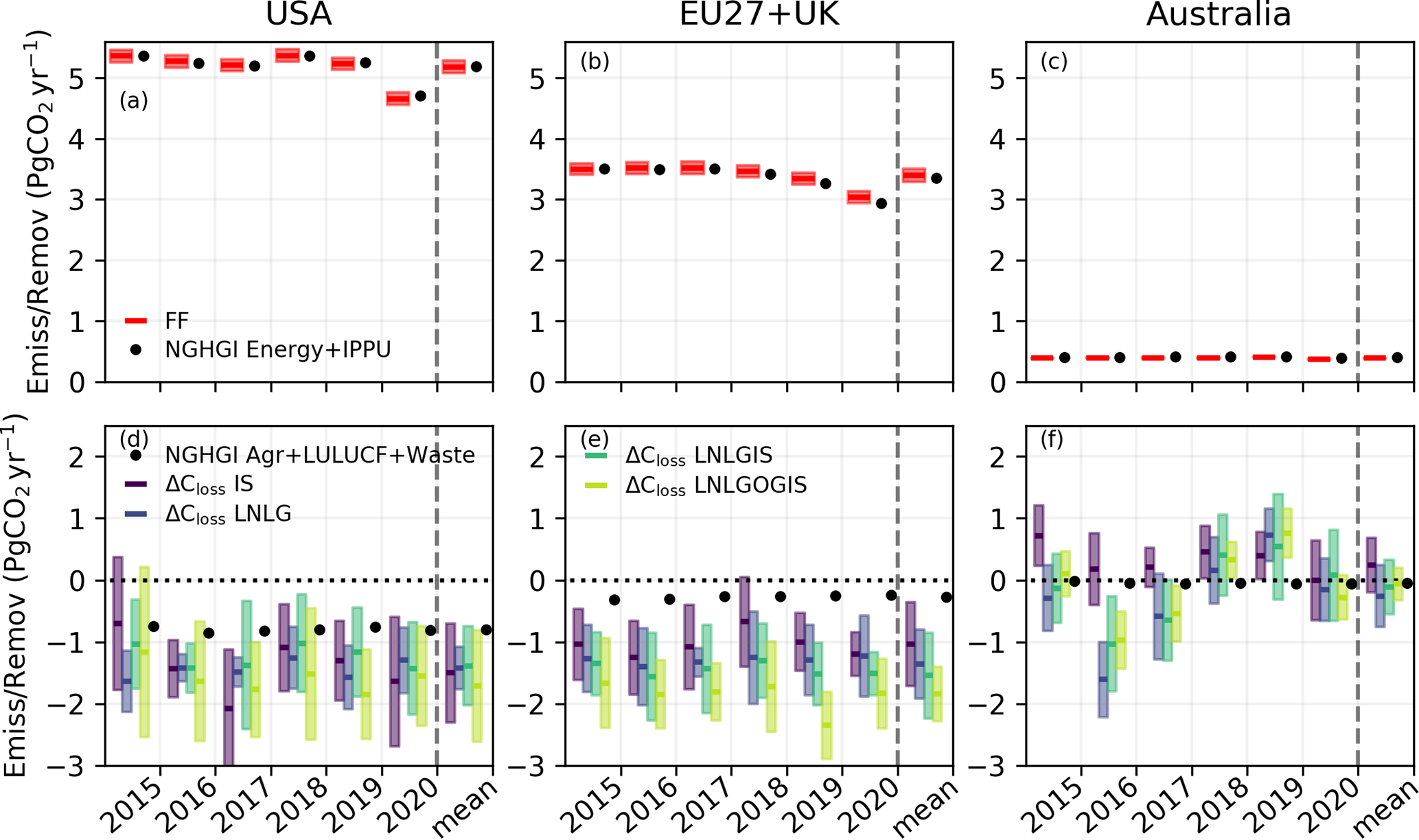
For this analysis, we compare NGHGIs and our dataset for three entities: the USA, European Union plus the United Kingdom (EU27+UK) and Australia. These were chosen for two reasons. First, NCE is better constrained by atmospheric CO2 data over these relatively large regions. This is reflected in the FUR metric, which gives values of 0.76–0.91 for the USA (meaning a 76 %–91 % uncertainty reduction), 0.38–0.51 for EU27 and 0.45–0.78 for Australia. Second, each of these entities has small unmanaged land areas, making this more of an apples-to-apples comparison. An area of 95 % of the USA is managed, with most unmanaged land being in the state of Alaska (Ogle et al., 2018). Similarly, all land in the EU27+UK is considered managed except for 5 % of France’s territory (Petrescu et al., 2021).
Figure 15 shows time series of emissions and removals from NGHGIs and Byrne et al. (2022) over 2015–2020. We focus our analysis on the 2015–2020 mean estimates, as top-down methods are expected to be more sensitive to IAV in the carbon cycle than NGHGI methods for individual years. Strong agreement is found between the NGHGI Energy+IPPU emissions and the fossil fuel emissions in Byrne et al. (2022), while larger differences are found between Agr+LULUCF+Waste and ΔCloss. Averaged over the 2015–2020 period, we obtain statistically significant differences between Agr+LULUCF+Waste and ΔCloss for the USA and EU27+UK for each experiment (based on Student’s t test at 0.05 significance level). In each case the top-down estimates suggest greater carbon sequestration by land, with mean differences of 0.59–0.91 Pg CO2 yr−1 for the USA and 0.99–1.79 Pg CO2 yr−1 for the EU27+UK. The reasons for these differences are unclear but are not expected to be explained by removals in unmanaged lands. It is possible that NGHGI methods miss or underestimate sink processes and/or that there are biases affecting the top-down estimates (see Sect. 9 for remaining challenges in top-down estimates). We encourage further research and comparison between the NGHGI and top-down research communities to better understand the sources of these differences.
Fuente: https://essd.copernicus.org