
Varios investigadores han estudiado las respuestas ionosféricas a diferentes eventos geofísicos naturales y artificiales utilizando GNSS y otros sensores de observación ionosféricos, pero siguen existiendo algunos problemas críticos. Una cuestión fundamental sobre las observaciones ionosféricas es cómo se pueden aislar las firmas detectadas a partir de un evento de fuente particular del ruido de fondo de la ionosfera. Debido a la naturaleza dinámica de la ionosfera, es crucial filtrar el ruido y otros efectos a través de un procesamiento de datos suficiente. Otra cuestión fundamental es si el TID detectado puede ser discriminado adecuadamente entre muchos eventos fuente. Si bien en algunos estudios [6,7] se observaron diferentes propiedades de los TID entre unos pocos eventos seleccionados, los análisis exhaustivos de muchos eventos son limitados. Recientemente, los algoritmos de Inteligencia Artificial (IA) han demostrado ser beneficiosos debido a su capacidad de procesamiento masivo de datos, reduciendo el potencial de errores humanos.
Ionospheric responses to various geophysical events have been studied for decades, as they can play a key role in triggering events. When geophysical events such as earthquakes, tsunamis, volcanic eruptions, magnetic storms, tropical storms, and large-scale explosions occur, gravity waves, gravity acoustic waves, or acoustic waves are generated and propagated along the lower and upper atmosphere.
Researchers have used various sensors to detect the signatures of these waves, which are traveling ionospheric disturbances (TIDs) [1-5]. Early and accurate detection of TIDs can provide valuable information on event origin and velocity of the produced waves. However, detecting TIDs is challenging because of the background ionospheric behaviors and the numerous sources that can trigger disturbances in the ionosphere. While various sensors have been used to monitor TIDs, the advent of GNSS has facilitated research development. As the ionosphere is a dispersive medium for GNSS signals, dual or multiple frequency GNSS signals can extract the total electron content (TEC) on a single line of sight. TIDs can be detected by analyzing TEC time series.
Although a number of researchers have investigated ionospheric responses to different natural and artificial geophysical events using GNSS and other ionospheric observing sensors, some critical problems remain. One fundamental question about ionospheric observations is how signatures detected from a particular source event can be isolated from the ionosphere’s background noise. Because of the ionosphere’s dynamic nature, it is crucial to filter out the noise and other effects through sufficient data processing. Another fundamental question is if the detected TID can be properly discriminated between many source events. While a few studies [6,7] showed different properties of TIDs between a few selected events, comprehensive analyses for many events are limited.
Recently, Artificial Intelligence (AI) algorithms have proven beneficial because of their capacity for massive data processing, reducing the potential for human errors. With the growing number of GNSS infrastructure including dense GNSS continuous operating reference stations (CORSs) on the ground and the enhanced space segment through multi frequency multi constellations, AI techniques become feasible for many GNSS research topics that includes ionosphere monitoring using GNSS, namely GNSS remote sensing. State-of-the-art AI applications to GNSS remote sensing have leveraged various AI techniques, but they mostly focus on TEC prediction [8], forecasting TEC disturbances [9] and detecting scintillation [10]. There has been limited work in induced TID detection that employs deep learning-
based anomaly detection methods [11].
Moreover, previous studies have detected TIDs induced by various historical events. Event induced waves detected in the ionosphere include the 2011 Tohoku, Japan earthquake [12] and following tsunami [13], the 2022 Tonga volcanic eruption [14] and non-natural hazards such as nuclear events [5]. Connecting a TID to a natural hazard event commonly relies on previous knowledge of the event and a human-lead search of station data to discover a potential detected TID induced by the event. This work aims to reverse these steps, detecting a TID from TEC time series data, potentially with the ability to precede the confirmation of a natural hazard event. In this study, we applied Long Short-Term Memory (LSTM) networks, a deep learning technique to detect ionospheric anomalies that can be considered as TIDs, and used different algorithms to relate them with their source event.

Approach: Deep Learning Based TID Detection
As a proof of concept for the automated TID detection method, we performed an experimental study using a test site in Alaska and processed a year-long dataset from 10 ground-based GNSS sites. Alaska is located in high latitudes where ionospheric anomalies may frequently appear due to not only natural hazards such as earthquakes but also other effects caused by geomagnetic storms or phase scintillations.
LSTM Based Anomaly Detection
Deep learning based anomaly detection uses deep learning neural networks to identify patterns in data and detect outliers. The basic idea is to train a neural network on a large dataset of normal data, and then use the trained model to identify any data points that deviate significantly from the learned pattern under normal conditions. This can be done using various deep learning neural network architectures. Recurrent neural networks (RNNs) are one type of neural network architecture that can model sequential data [15] for anomaly detection. RNNs are based on a feedforward network and include a mechanism that can retain past information to forecast future values [16]. LSTM is a type of RNN [17] capable of learning long term dependencies and are robust against the vanishing and exploding gradient problem of conventional RNNs [18]. LSTMs selectively remember or forget information over long time intervals, which makes them useful for tasks that involve sequential data. Recent studies applied LSTM methods to predict the ionospheric F2 parameter [8], disturbances during geomagnetic storm periods [19] and scintillations [20].
For TEC anomaly detection in this project, we used the 15 second sampling rate GNSS observations to obtain TEC values with 15 second sampling intervals. To avoid the impact of satellite geometry changes, solar activities and biases, the trend of TEC time series is removed and the remaining detrended TEC (dTEC) is used as input features. The input sequence of 15-minute-long TEC data—which is equivalent to 60 time steps—is used to predict the next value of TEC, or the next 15 second sample point. The input sequence was fed into a two-layer LSTM network with 256 neurons in each hidden layer, followed by two fully connected layers each with 128 neurons. The LSTM was trained for 25 epochs and used a scheduled learning rate from 1e-3 to 1e-6, reducing at epochs 10, 15 and 20. The batch size was set to 64. The loss function used to train the model was mean squared error (MSE). The final architecture was obtained by reaching the lowest MSE scores on the training data.
Error Processing and Analysis
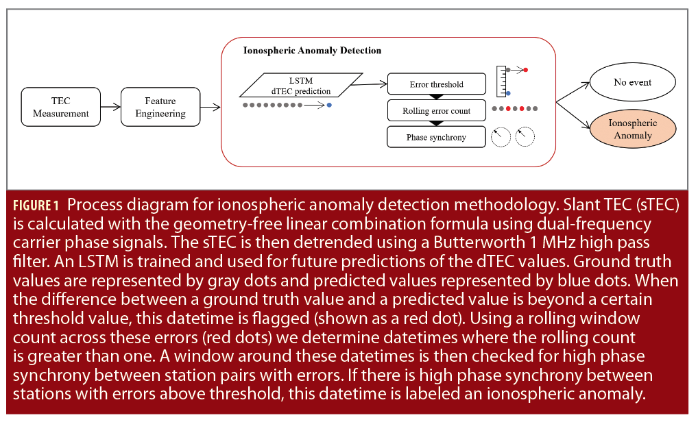
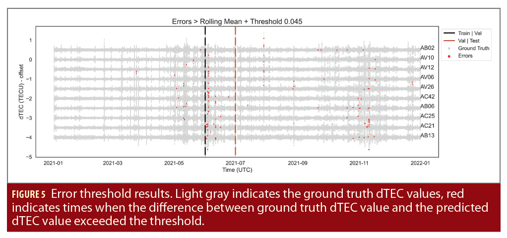
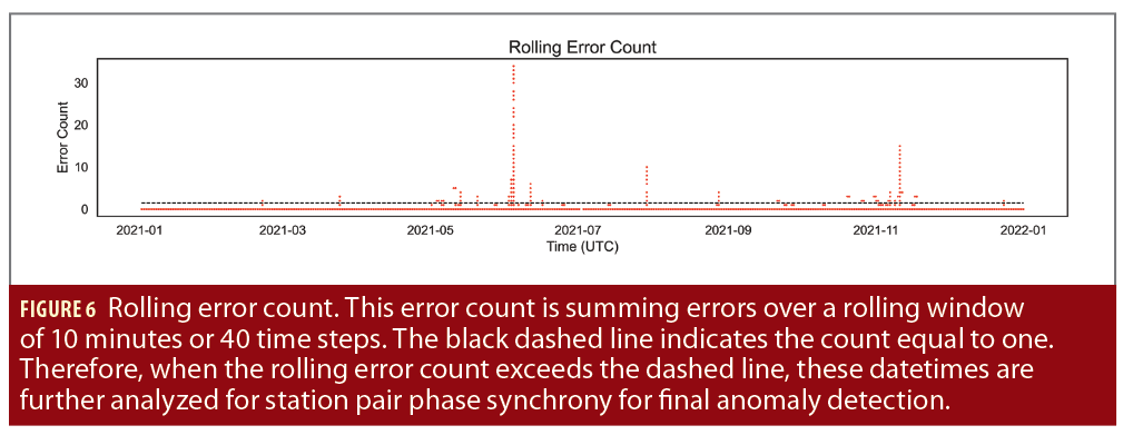
An error threshold is set by combining a rolling MSE with a multiple of the MSE standard deviation. This dynamic threshold was chosen to aid in managing day-to-day variations in dTEC measures. The number of errors within a rolling time window reflects the extent of the possible disturbance. Therefore, as MSEs are processed, we use a rolling MSE error count over 10-minute windows (or 40-time steps). If we observe more than one error within the rolling window, we then pull the data starting 10 minutes prior to when the error count exceeded one and end when the error count drops back below or equal to one. This slice of the data is then looped through each station-station pair (for 10 stations, this is 45 unique pairs) to measure phase synchrony between each pair, accounting for lag. If phase synchrony exceeds 0.9, a high synchrony level, among stations during times of observed errors then we label the resulting date time slice an ionospheric anomaly, with the time of the first observed anomaly as the time of when the error count exceeded one.
Phase synchrony is calculated between two station pairs with Equation 1 where the angle of the dTEC value is the Hilbert Transform of the dTEC. In Equation 1, φsyn is the phase synchrony between two stations, φ1 is the dTEC phase angle of the first station and φ2 is the dTEC phase angle of the second station.
![]()
Experiments
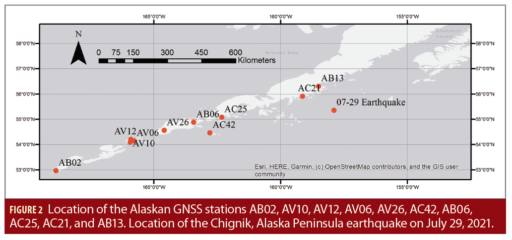
On July 29, 2021, there was a Mw 8.2 earthquake reported south of Perryville, Alaska. We applied the proposed approach and attempted to verify the method by checking if the algorithm could detect the TID associated with the earthquake.
GNSS observations were obtained from UNAVCO for 10 stations: AB02, AV10, AV12, AV06, AV26, AC42, AB06, AC25, AC21, and AB13, between latitudes of 52°-57°N and longitudes of 158°-169°W. Corresponding broadcast navigation files were obtained from the National Oceanic and Atmospheric Administration (NOAA) Continuously Operating Reference Station (CORS) Network (NCN) data archive. These stations are located along the Alaska Peninsula and Aleutian Islands. They were chosen for their nearly complete observations each day in 2021 (Figure 2).
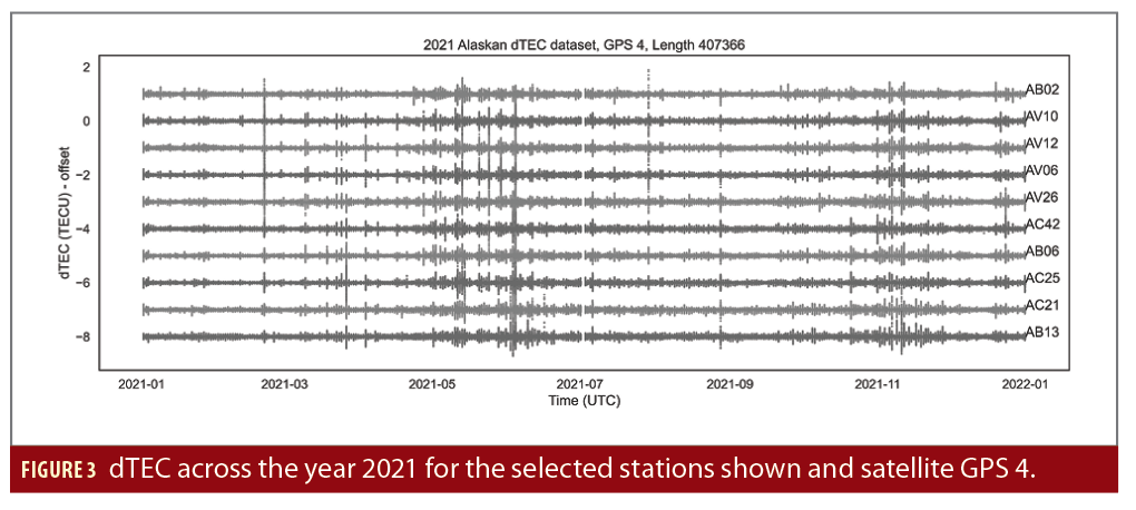
Slant TEC (sTEC) measurements were calculated with the geometry-free linear combination formula using dual-frequency carrier phase signals [21] between these stations and satellite GPS 04, part of the GPS Block III iteration. The line of sight between these stations and GPS 04 crosses the Gulf of Alaska and Pacific Ocean, south of the stations, a location with high levels of tectonic activity. An elevation angle cut off was set to 20 to remove edge effects. To improve detection results, sTEC data was filtered using the fourth-order Butterworth high pass filter to remove frequencies below 1 MHz. The resulting data is now labeled as dTEC.
The final dTEC data set, after removing NaN values, resulted in a time series length of 407,366 for the entire year of 2021, for each station-satellite pair (Figure 3). The data set was divided into training, validation and test data sets. Training data included January through the end of May, validation included June, and test data included July through the end of December. All data was normalized for LSTM training and testing purposes.
Results
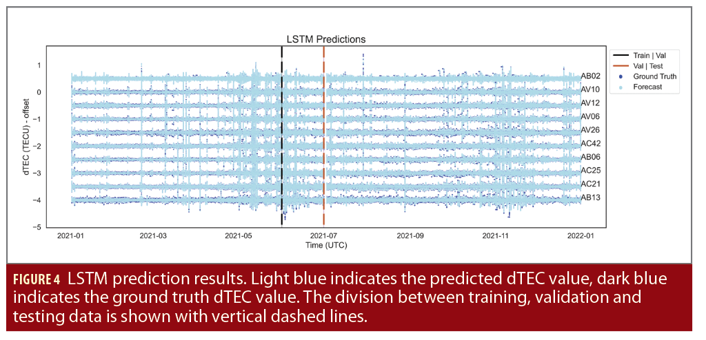
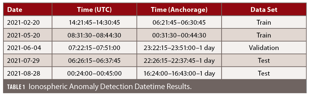
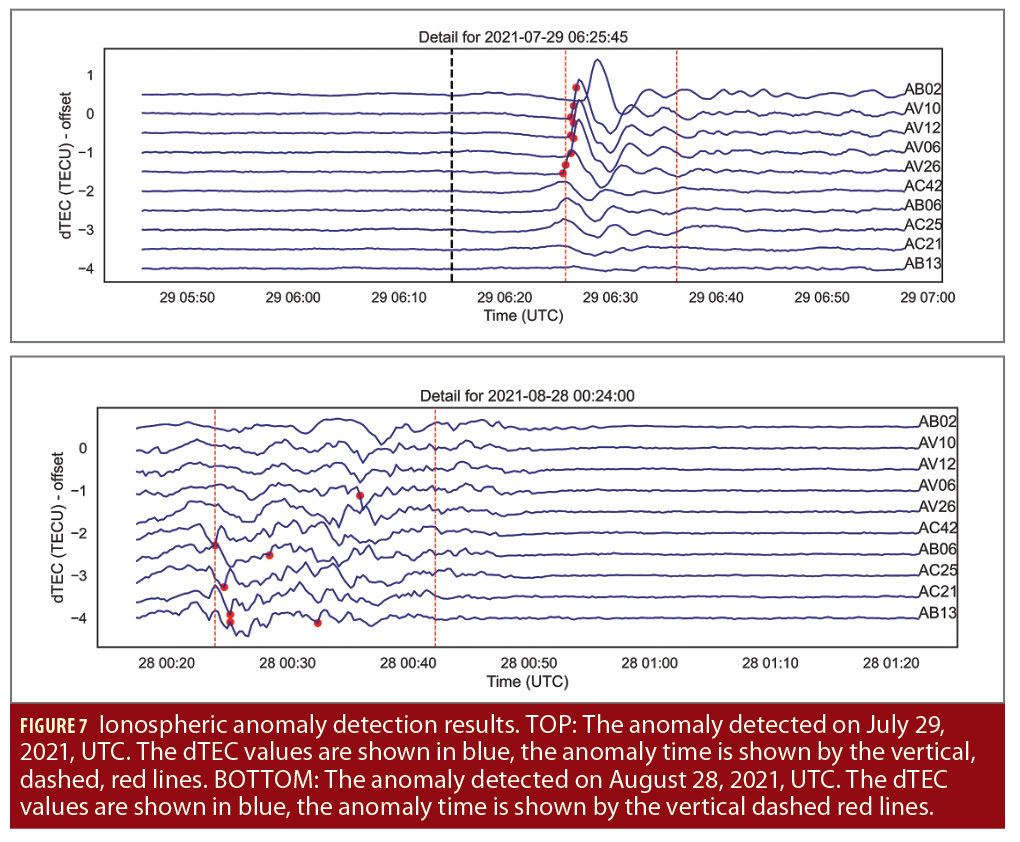
The LSTM prediction results capture the temporal dynamic of the dTEC values across the 10 stations (Figure 4). Therefore, using this model for predicting error anomaly detection is valid. A total of 141 errors were detected across 43 days using the error thresholding technique (Figure 5). Five date times exceeding a rolling error count of one (Figure 6) with station pairs exhibiting high phase synchrony during flagged errors were detected. These five datetimes are listed in Table 1.
The ionospheric anomaly detected starting July 29, 2021, at 06:26:15 (UTC) exhibited errors above threshold across four nearby stations, at the southwestern most location of stations in this study. The same four stations plus two additional ones also exhibited high phase synchrony during the same time as their errors. This anomaly datetime is roughly 10 minutes after the Chignik, Alaska Peninsula earthquake, which occurred on July 29, 2021, at 06:15:49 (UTC) according to the U.S. Geological Survey National Earthquake Information Center (USGS-NEIC). This magnitude 8.2 earthquake was located at 55.364°N 157.888°W, at a depth of 35.0 km.
The ionospheric anomaly detected at datetime starting on August 28, 2021, at 00:24:00 (UTC) exhibited errors above threshold at four stations with non-overlapping high phase synchrony between two station pairs. As of the time of publication, this anomaly source has not been identified.
Summary and Discussion
Detecting ionospheric disturbances is an important undertaking in geolocation, particularly with respect to natural hazards like earthquakes and tsunamis, as well as anthropogenic hazards such as nuclear and ballistic weapons tests. These ionospheric disturbances are often reflected in TEC after proper signal processing such as detrending (dTEC in our study), but detecting TID as they occur is an open area of interest in geolocation research. In this article, we implemented a deep learning model using the LSTM architecture to predict dTEC for 2021 from data across 10 stations in Alaska. We then used the error threshold, error count and phase synchrony methods to identify timesteps in the dTEC data where the measurements are potentially natural hazard induced TID. Because we expect the LSTM to accurately predict “normal” dTEC behavior, large disparities between the prediction and the measured dTEC should theoretically indicate the presence of an anomaly related to an event such as an earthquake.
We compared the LSTM dTEC prediction error with the prediction error generated by a naive forecaster (i.e., a predictor that predicts the value at time t+1 to be equal to the value at time t). The LSTM outperformed the baseline by six times with respect to mean squared error on the test data. This indicates a significant improvement over the naive model. Of the two ionospheric anomalies identified in 2021 with this method, one was the result of the magnitude 8.2 earthquake and the other unknown. Based on these results, we conclude the LSTM anomaly detection method is a viable option for further contributions to automate TID detection across long term observations in the North America region.
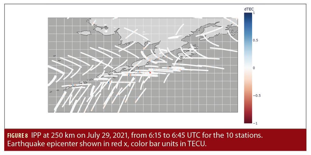
Using an ionospheric pierce point (IPP) of 250 km, based on Incoherent Scatter Radar (ISR) observation of ionosphere altitude at this time, we observe pierce points over the Gulf of Alaska, with station AB06 IPP directly over the earthquake epicenter (Figure 8). From Figure 8 we observe dTEC amplitude increase starting from the earthquake epicenter along a vector southwest, roughly parallel to the coastline, with amplitudes increasing from +/- 0.25 dTEC (TECU) to +/- 0.90 dTEC (TECU) along this path.
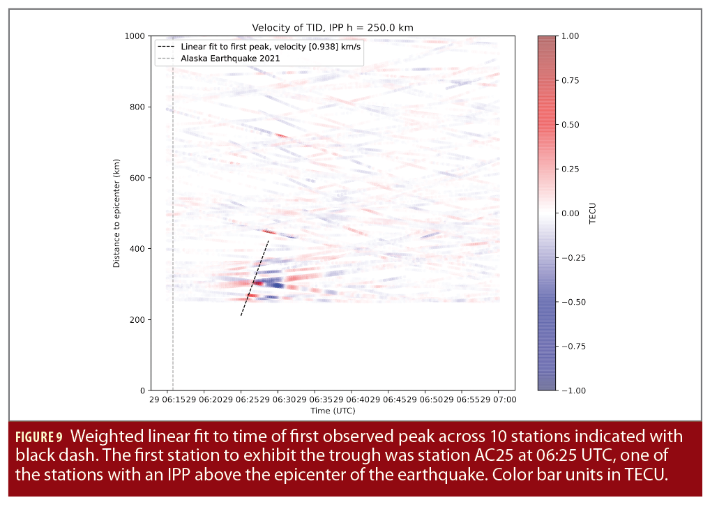
Plotting IPP distance to earthquake epicenter over time, and the time of first peak (Figure 9), we can use a weighted linear fit, weighted by absolute amplitude values, to determine the velocity of the disturbance. This results in an approximate 1 km/s velocity of what is likely an induced TID by the Chignik earthquake event.
An additional and important area of continued research is the ability to identify the cause of these detected ionospheric anomalies. We plan to continue working on developing a method that can classify the results of these detected ionospheric anomalies, predicting the potential source.
References
(1) Donn, W. L., and M. Ewing (1962), Atmospheric waves from nuclear explosions—Part II: The Soviet test of 30 October 1961, J. Atmos. Sci., 19(3), 264–273, https://doi.org/10.1175/1520-0469(1962)019<0264:AWFNEI>2.0.CO;2
(2) Fuller-Rowell, T., M. Codrescu, R. Moffett, and S. Quegan (1994), Response of the thermosphere and ionosphere to geomagnetic storms, J. Geophys. Res., 99(A3), 3893–3914. https://doi.org/10.1029/93JA02015.
(3) Vadas, S. L., and G. Crowley (2010), Sources of the traveling ionospheric disturbances observed by the ionospheric TIDDBIT sounder near Wallops Island on 30 October 2007, J. Geophys. Res., 115, A07324, https://doi.org/10.1029/2009JA015053.
(4) Park, J., R. R. B. von Frese, D. A. Grejner-Brzezinska, Y. Morton, and L. R. Gaya-Pique (2011), Ionospheric detection of the 25 May 2009 North Korean underground nuclear test, Geophys. Res. Lett., 38, L22802, https://doi.org/10.1029/2011GL049430.
(5) Park, J., J. Helmboldt, D. A. Grejner-Brzezinska, R. R. B. von Frese, and T. L. Wilson (2013), Ionospheric observations of underground nuclear explosions (UNE) using GPS and the Very Large Array, Radio Sci., 48, https://doi.org/10.1002/rds.20053.
(6) Kirchengast, G., K. Hocke, and K. Schlegel (1995) Gravity waves determined by modeling of traveling ionospheric disturbances in incoherent-scatter radar measurements.
(7) Park, J., D. A. Grejner-Brzezinska, R. R. B. von Frese, and Y. Morton (2014), GPS discrimination of traveling ionospheric disturbances from underground nuclear explosions and earthquakes, Navigation, 61: 125–134. https://doi.org/10.1002/navi.56.
(8) Moon, S., Kim, Y. H., Kim, J.-H., Kwak, Y.-S., and Yoon, J.-Y. (2020). Forecasting the ionospheric f2 parameters over jeju station (33.43°N, 126.30°E) by using long short-term memory. Journal of the Korean Physical Society, 77(12), 1265–1273. doi:10.3938/jkps.77.1265
(9) Iluore, K. and Lu, J. (2022). Long short-term memory and gated recurrent neural networks to predict the ionospheric vertical total electron content. Advances in Space Research, 70(3), 652–665. doi:10.1016/j.asr.2022.04.066
(10) Liu, Y. and Morton, Y. J. (2020). Automatic detection of ionospheric scintillation-like gnss satellite oscillator anomaly using a machine-learning algorithm. Navigation (Washington), 67(3), 651–662. doi:10.1002/navi.385
(11) Luhrmann, F., Park, J., Wong, W., Corcoran, F., and Lewis, C. (2022). Detecting traveling ionospheric disturbances with lstm based anomaly detection. Proceedings of the 35th International Technical Meeting of the Satellite Division of The Institute of Navigation (ION GNSS+2022), Denver, Colorado, September 2022, pp. 3002-3011.
(12) Chen, Saito, A., Lin, C. H., Liu, J. Y., Tsai, H. F., Tsugawa, T., Otsuka, Y., Nishioka, M., & Matsumura, M. (2011). Long-distance propagation of ionospheric disturbance generated by the 2011 off the Pacific Coast of Tohoku earthquake. Earth, Planets, and Space, 63(7), 881–884. https://doi.org/10.5047/eps.2011.06.026
(13) Tang, Zhang, X., & Li, Z. (2015). Observation of ionospheric disturbances induced by the 2011 Tohoku tsunami using far-field GPS data in Hawaii. Earth, Planets, and Space, 67(1), 1–7. https://doi.org/10.1186/s40623-015-0240-0
(14) Themens, Watson, C., Zagar, N., Vasylkevych, S., Elvidge, S., McCaffrey, A., Prikryl, P., Reid, B., Wood, A., & Jayachandran, P. T. (2022). Global propagation of ionospheric disturbances associated with the 2022 Tonga volcanic eruption. Geophysical Research Letters, 49(7), n/a–n/a. https://doi.org/10.1029/2022GL098158
(15) Brownlee, J. Deep Learning for Time Series Forecasting: Predict the Future with MLPs, CNNs and LSTMs in Python. N.p., Machine Learning Mastery, 2018.
(16) Rumelhart, Hinton, G. E., & Williams, R. J. (1985). Learning Internal Representations by Error Propagation. in Parallel Distributed Processing: Explorations in the Microstructure of Cognition: Foundations , MIT Press, 1987, pp.318-362.
(17) Hochreiter, & Schmidhuber, J. (1997). Long Short-Term Memory. Neural Computation, 9(8), 1735–1780. https://doi.org/10.1162/neco.1997.9.8.1735
(18) Sak, Senior, A., & Beaufays, F. (2014). Long Short-Term Memory Based Recurrent Neural Network Architectures for Large Vocabulary Speech Recognition. Françoise Beaufays, CoRR, vol. abs/1402.1128
(19) Kim, J.-H., Kwak, Y.-S., Kim, Y., Moon, S.-I., Jeong, S.-H., & Yun, J. (2021). Potential of regional ionosphere prediction using a long short-term memory deep-learning algorithm specialized for geomagnetic storm period. Space Weather, 19, e2021SW002741. https://doi.org/10.1029/2021SW002741
(20) Zhang, H., Wang, F., Sheng, D., Ban, P., & Liu, Y. (2022). Precursors Identification for Forecasting UHF-Band Ionospheric Scintillation Events Over Chinese Low-Latitude Region by Deep Learning. Earth and Space Science (Hoboken, N.J.), 9(9). https://doi.org/10.1029/2021EA002164
(21) Hofmann-Wellenhof, B.; Lichtenegger, H. ; Wasle, E. GNSS—Global Navigation Satellite Systems, 1st ed.; Springer Vienna: Vienna, 196 Austria, 2007.
Dr. Jihye Park is an associate professor of Geomatics in the School of Civil and Construction Engineering at Oregon State University. Dr. Park holds a Ph.D. in Geodetic Science and Surveying from The Ohio State University. Her research interests include GNSS positioning and navigation, GNSS remote sensing, GNSS meteorology, and GNSS-Reflectometry for monitoring the Earth’s environments, natural hazards, as well as artificial events.
Fiona Luhrmann is a research graduate assistant at the College of Engineering pursuing a Ph.D. of Geomatics Engineering and a minor in Artificial Intelligence at Oregon State University. Her research interests are machine learning applications in GNSS signal processing and atmospheric monitoring.
Dr. Weng-Keen Wong is a Professor in the School of Electrical Engineering and Computer Science at Oregon State University. He received his Ph.D. (2004) and M.S. (2001) in Computer Science from Carnegie Mellon University, and his B.Sc. (1997) from the University of British Columbia. His research areas are in data mining and machine learning, with specific interests in anomaly detection, probabilistic graphical models, computational sustainability, and explainable artificial intelligence.
Fuente: https://insidegnss.com