
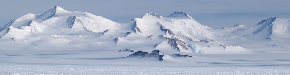
Encuentran en la Antártida el punto terrestre más profundo del planeta. Se inician así otros estudios tales como que sucederá en el futuro con los glaciares.
Description
The data are in one single file in NetCDF format (795 Mb) and all heights are in meters above mean sea level (the geoid used is provided in the NetCDF file). All the data use the same 450 m-resolution grid although the “true” resolution of the bedrock may vary depending on the method used to map the bed. This dataset uses data from 1993 to 2016 and has a nominal date of 2012 (same as REMA).
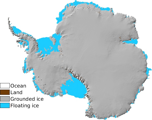 |
Antarctic mask The ice/land masks are from ADD rock outcrop, and the floating ice is derived from InSAR grounding lines (pers. comm.). 0 = ocean, 1 = ice-free land, 2 = grounded ice, 3 = floating ice, 4 = lake Vostok |
 |
Surface elevation The surface dem is from REMA. |
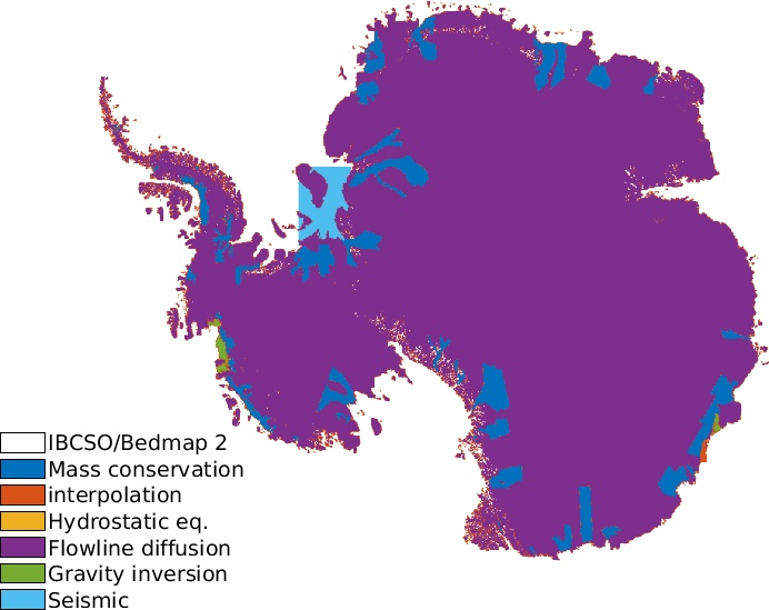 |
Source Method used to calculate ice thickness: 0 = none, 1 = REMA/IBCSO, 2 = Mass conservation, 3 = interpolation, 4 = hydrostatic equilibrium, 5 = streamline diffusion, 6 = gravity, 7=seismic, 10+ = bathymetry data |
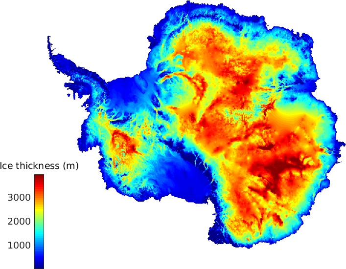 |
Ice thickness The ice thickness is inferred using mass conservation along the peryphery of the ice sheet and ordinary kriging in the interior. |
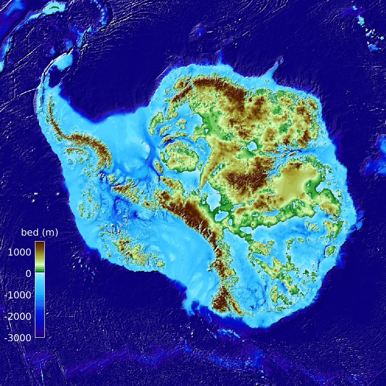 |
Bed topography The bed elevation is calculated by subtracting the ice thickness from the surface elevation data. |
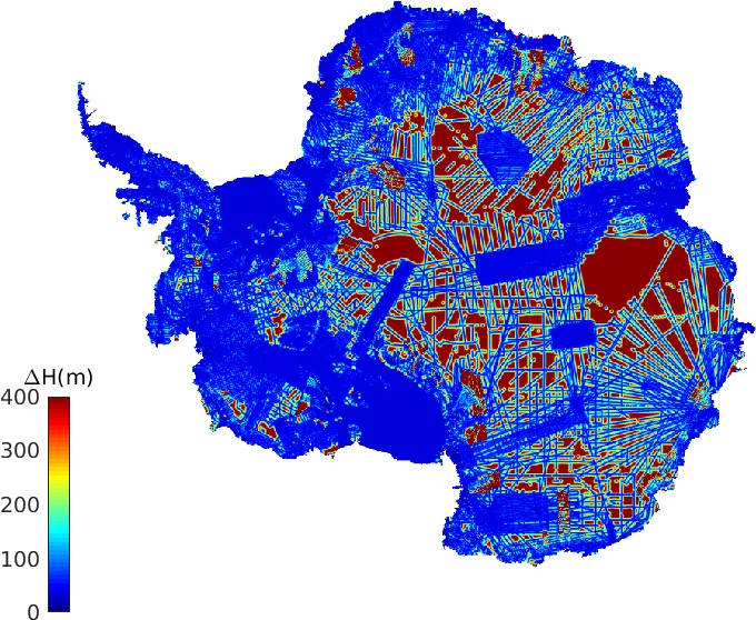 |
Error map Ice thickness and bed topography error. |
For the hydrostatic equilibrium calculation, we used a density of ice ρice=917 kg/m3, and an ocean water density of ρocean=1027 kg/m3 (following the densities used in Griggs & Bamber 2011 and Chuter & Bamber 2015).
As any model output, there are errors in these maps (there is an estimate included in the dataset). Feedback is more than welcome.
Citation
Morlighem, M., Rignot, E., Binder, T. et al. Deep glacial troughs and stabilizing ridges unveiled beneath the margins of the Antarctic ice sheet. Nat. Geosci. (2019) doi:10.1038/s41561-019-0510-8
Disclaimer
The ice thickness and bed topography are model outputs and are not free of error (especially in regions where ice thickness measurements are sparse). This dataset is a work in progress and we encourage users to send us feedback so that we keep improving it.
Projection
The projection is Polar Stereographic South (71ºS, 0ºE), which corresponds to ESPG 3031
Reading with MATLAB
MATLAB now has an extensive library for NetCDF files.
filename = 'BedMachineAntarctica-2019-09-04.nc';

x = ncread(filename,'x');

y = ncread(filename,'y');

bed = ncread(filename,'bed')'; %Do not forget to transpose (MATLAB is column oriented)

%Display bed elevation

imagesc(x,y,bed); axis xy equal; caxis([-1000 3000]);
Converting heights to WGS84
All heights are referenced to mean sea level (using the geoid EIGEN-6C4). To convert the heights to heights referenced to the WGS84 ellipsoid, simply add the geoid height:
zellipsoid=zgeoid+geoid
Surface height and firn depth correction
All the quantities provided in BedMachine are in ice equivalent. This affects primarily the upper surface of the ice, to which we have subtracted a firn depth correction to account for the presence of air in the firn layer. The ice thickness is also in ice equivalent. To recover the top of the surface dem from RAME in WGS84:
zREMA=surface+firn+geoid
where “firn” is the firn depth correction, “surface” is the surface height, and “geoid” is the geoid height. All these quantities are provided in the netCDF file.
Acknowledgements and References
This project is performed at the University of California Irvine under a contract with the National Aeronautics and Space Administration (Sea Level Rise Program #NNX14AN03G and MEaSURES-3) and the National Science Foundation (Thwaites #1739031).
The ice thickness data are from:
- Gogineni, P. CReSIS RDS Data (from 2002 to 2017); freely available here http://data.cresis.ku.edu/.
- more to come…
Fuente: https://sites.uci.edu